
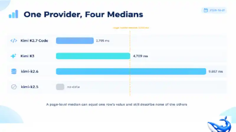
The OrcaRouter Kimi API page carries four rows and a header that says Median p50 4,709 ms [OURS]. Read the whole page and the number turns out to be one of the four rows’ own values, printed again at the top — Kimi K3 reports 4,709 ms in its own latency record [OURS].
That coincidence is not a bug. It is what a median does when the sample is small, and this page is a compact demonstration of a habit that costs teams real money: reading a page-level latency figure as though it described every row underneath it. On this provider, the row values run from 2,795 ms to 9,657 ms, a spread of 3.45×, and one of the four rows has no measurement at all.
The four rows, as measured
| Model | Row p50 | Row p95 | Input / output per 1M |
| Kimi K2.7 Code | 2,795 ms | 9,090 ms | $0.950 / $4.00 |
| Kimi K3 | 4,709 ms | 10,000 ms | $3.00 / $15.00 |
| `kimi/kimi-k2.6` | 9,657 ms | 10,000 ms | $0.950 / $4.00 |
| `kimi/kimi-k2.5` | no data | 1,000 ms | $0.600 / $3.00 |
All four p50 values are our own rolling telemetry over production traffic through the gateway [OURS]; the rates are the provider’s published prices passed through with $0 markup [VENDOR]. The 10,000 ms figures in the p95 column are the reporting ceiling, not a measurement — the figure saturates there rather than describing a distribution that happens to end at ten seconds.
Two of those rows deserve a second look before anything else in this article.
K2.7 Code and k2.6 cost exactly the same. $0.950 in, $4.00 out, both with a 262K context window. If you were picking between them on price you would find nothing to pick on, and if you picked on the page header’s 4,709 ms you would be reading a number that belongs to neither. Their measured p50 differs by 6,862 ms — 3.45× — on identical rates.
The p95 column saturates. Three of the four rows read 10,000 ms at p95. That does not mean three of four models are equally slow — it means the reporting window caps there. When a distribution’s 95th percentile sits exactly on the ceiling, you have learnt that at least 5 percent of requests were slow, not how slow; the useful reading is in the p50, plus the fact that three of the four rows hit the cap.
Why the page median equals one row
The header statistic is computed over the provider’s traffic, and on a four-row catalogue the arithmetic of a median is unforgiving.
Three of the four rows carry a measured p50: 2,795, 4,709 and 9,657. The middle of those three is 4,709, which is K3’s own figure, and that is exactly the number the header prints. The fourth row has no measurement and therefore contributes nothing to the middle.
So the page median is not an average of four models and it is not an independent statistic. It is the middle observation of a three-value set, and it happens to be a value one of the models already reports. On a longer catalogue that coincidence would be unlikely; on a four-row catalogue with one gap it is close to inevitable.
That is the general hazard. On a catalogue with 76 rows, a page median is a decent summary of a population. On a catalogue with four, it is one model’s number wearing a page-level label. Nothing about the page is misleading — it prints the row values in the same table — but a reader who takes the header away and quotes it as “the provider’s latency” has quoted one row out of three.
The same structural accident shows on other catalogues for the same reason. The Grok page’s header reads 8,000 ms; only one of its five rows carries a measured p50, and that row is Grok 4.6 at 8,000 ms [OURS]. The Z.ai page’s 3,415 ms is GLM 5.3’s row value. Where a catalogue has one dominant-traffic row, the page median is that row’s median.
What a 6,862 ms gap does to a pipeline
The useful question is not which number is right. It is what the difference costs when you put models in series.
A two-step chain — retrieve with one model, verify with another — waits for both legs. Its latency is not the average of the two p50s; it is closer to the sum, and the slow leg dominates. Pair K2.7 Code at 2,795 ms with k2.6 at 9,657 ms and the chain’s floor is about 12.5 seconds before any generation time is counted. Pair K3 with itself and the floor is 9.4 seconds.
That is the arithmetic that makes a catalogue page more useful than a single model page: the spread is the thing you design around, and it is only visible when the rows are side by side. A team that bought one model and measured it once would never see the 6,862 ms, because they would never have run the other row.
There is a second, quieter reading in the same table. The two slowest rows are not the most expensive ones. k2.6 at 9,657 ms costs $0.950 in, while K3 at 4,709 ms costs $3.00 — more than three times as much per input token and half the latency. If response time is a product requirement, the page is telling you that the expensive row is the fast one here, which is the opposite of the usual assumption that premium models are slower.
What the capability row adds
All four models carry the same four capability flags: Vision, Tools, Reasoning and JSON mode, 4 of 4 [OURS]. That is the tidiest capability distribution of any provider catalogue on the site, and it removes one of the usual tiebreakers. You cannot choose between K2.7 Code and k2.6 on features; both support everything the page tracks. Price does not separate them either. What separates them is latency, and latency is the one column the page header summarises badly.
The catalogue’s own framing reinforces the point: the header names K3 in its playground call to action — “Try Kimi K3 in the playground” — and K3 is the row whose median the header statistic reproduces. The page is leading with its flagship. That is a merchandising decision rather than a measurement, and it is worth knowing which is which when you quote the number.
How to read a latency column
Four habits, each cheap, each derived from something visible on this page.
Compare rows, not headers. A page-level median answers “what does this provider feel like on average”, which is a question nobody asks in production. The row values answer “what will this call feel like”, which is the question every pipeline actually has.
Find the saturation point before you trust a percentile. Three of these four rows read exactly 10,000 ms at p95. A percentile that lands on a round ceiling is a censored value: you know the tail exists, not how far it extends. If your timeout policy is derived from a p95 like that, you are deriving it from the reporting limit.
Treat “no data” as a third value, not as zero. `kimi/kimi-k2.5` shows no p50 and a p95 of 1,000 ms. A missing p50 is not a fast model; it is a model with too little traffic in the window to compute one. Any sort that puts a missing value at the top will put an unmeasured row ahead of a measured one.
Price and latency are independent columns, and on this page they point in opposite directions. The cheapest row by input rate is the one with no measurement; the most expensive is the second fastest; the two same-priced rows are 3.45× apart. That is not an anomaly, it is normal — and it is why choosing on price alone and choosing on latency alone produce different shortlists.
A catalogue page is worth reading precisely because it lets you see the disagreement. One model page tells you what one model does; four rows side by side tell you what the choice costs. See more